1+1=3

This is, of course, an extremely old trick in Excel which I use to try and generate some interest in spreadsheets when teaching at the sleepy 3pm slot.



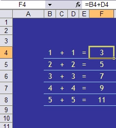
The formula for F4 looks fine, so why on earth does it show the wrong answer?

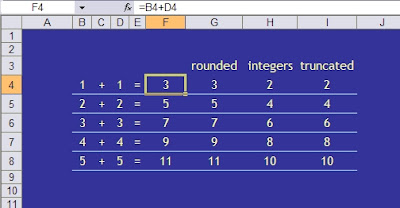
It's all to do with the difference between what Excel knows and what Excel shows. The figures above have had their decimal display adjusted so the display is rounded to the nearest whole number. In fact the data in B4 and D4 is 1.4 and in F4 Excel calculates 2.8

Whilst this may seem either stupid to do in the first place, obvious or generally something you don't need me to tell you about, problems can arise when, for example, dealing with money. You may well not notice that costs from some other calculations, rounded to the nearer penny, actually add up to a different total than the figure Excel shows as a total. Excel will add the exact figures (calculating up to 15 decimal places) and then round the total to the nearer penny - not necessarily the same thing. In an RSA OCR spreadsheet exam many years ago this occurred and only one out of hundreds of students spotted it and asked me what to do.

If you prefer to have 1 and 1 making 2, and totals of displayed figures adding up to the same figure as you'd get from good old mental arithmetic, counting on fingers or even an old calculator, then you'll need to tell Excel what you want.

There are three useful formulae:
=ROUND() does what Excel does naturally when you change the decimal display, rounding to the nearest number of digits indicated
=INT() may be more useful, displaying just the whole number
=TRUNC() is the best option, restricting the number stored to a chosen number of digits.




You could now, for example add up column H or I and get 30 using the usual sum formula. It is important to apply the formula at the right stage of a calculation but this might help avoid less obvious but potentially costly or embarrassing errors.